The relationship between changes in the money supply and growth has been a very important subject for a decade.
A concrete example from well-known economic theories allows us to understand them…
As soon as the Böhm-Bawerk’s peasant sells his harvest on the market in neighboring town, he buys a plow (to increase his production, productivity and profits) from the seller of agricultural equipment who orders 2 plows from his supplier who orders plowshares from the blacksmith who orders steel, and so on.
Money flows quickly between them and everyone works and earns money.
During the following years, the Böhm-Bawerk’s peasant continues to reinvest his profits into productive capital and everyone in the area does the same.
Then banks and savings banks open agencies that make money flow even faster between those who do not have investment projects and investors who are short of capital.
So, Böhm-Bawerk’s peasant can borrow money too from his bank to buy a tractor without having to wait to have enough savings to finance his purchase.
So all was going fine for all these people. But one day, politicians wanted to make them pay new taxes by claiming that it would bring them benefits.
The Böhm-Bawerk’s peasant, suspicious, does not trust these projects that worry him.
Instead of investing again, he prefers to increase his savings to face a foreseeable deterioration of his situation and everyone in the area reacts like him.
Consequently, money is no longer circulating, or almost no more. The (precautionary) savings increase.
Customers from the Böhm-Bawerk’s peasant buy less from him, and so do all other entrepreneurs.
Production stagnates, as well as incomes and the situation is likely to worsen even to degenerate into a crisis.
It’s simple.
Everything is simple, as Milton Friedman said and said again. He did not understand why people did not understand monetarism. Let us transpose this simplified history into macroeconomic concepts…
Only United States provide series of data on the long period (since 1959) that can easily be downloaded (thanks to our friend Fred of Saint Louis), particularly on monetary aggregates, so that monetary problems can be studied on a reliable basis.
Deposits of (US) households in savings banks are recorded in the M2-M1 aggregate.
It is clear from this first graph that real GDP growth increases as M2-M1 decreases, and vice versa, which is the perfect macroeconomic transposition of the behavior of the Böhm-Bawerk’s peasant,
Document 1:
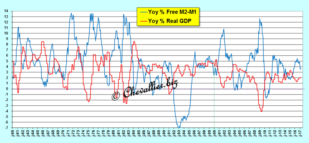
More precisely, it is not exactly the change in the M2-M1 aggregate (from year to year as a percentage) that causes the opposite direction of real GDP growth to change, but the difference between this change in the M2-M1 aggregate and that of the growth rate of real GDP, i.e. what I call the free money supply.
The most important is the difference between the rate of real GDP growth and the change in household savings: if they increase their savings more than their real incomes, GDP growth falls, and vice versa.
This rule is better checked over the more recent period, starting in 2000, i.e. after the period of large inflation during the 70’ and then of disinflation, which makes it possible to demonstrate it a posteriori…
Document 2:
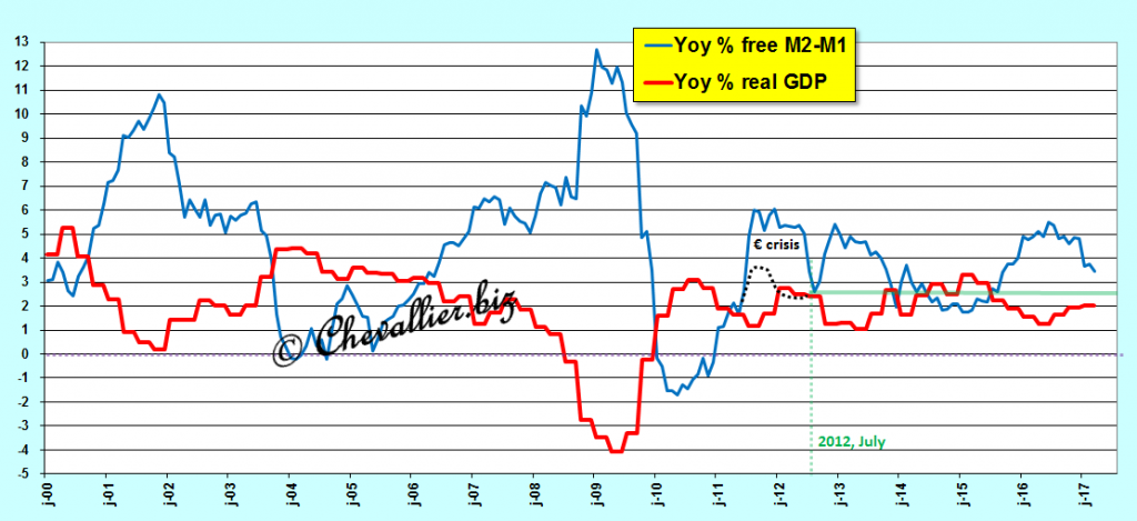
From 2000, Pearson correlation coefficient is -0.8 (more precisely -0.76), that confirms undoubtedly this negative correlation which is even better from August 2012: -0.9 (more precisely -0.88!) because euro-system crisis in 2011 have had anxiogenic repercussions of an exogenous event in USA.
So, Americans increased their savings but the GDP did not decrease because this happened abroad,
Document 3:
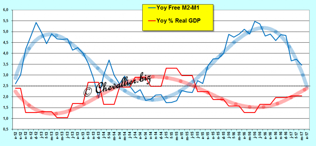
From August 2012, polynomial curves show that the economic fundamentals are right in USA.
So, this rule of free money supply is well verified, and even it is able to know the evolution of Americans behaviors with 10 days of lag, the figures of the monetary aggregates (of the week ending the Monday of the previous week) being published on Thursday evening by the Fed, which makes it possible to well anticipate changes in GDP, all other things being equal,
Document 4:
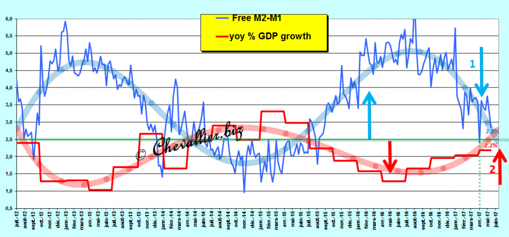
The critical value of these rates is 2.5% (year-on-year), i.e. as the real GDP growth rate equals the increase in the free money supply.
The real GDP growth rate is then at its optimal potential at 2.5% when the rate of increase of the M2-M1 aggregate is at 5.0%.
Indeed, in this case, the increase in the free money supply is also 2.5%, i.e. the difference between the rate of increase of the M2-M1 aggregate of 5.0% and (minus) the real GDP growth rate.
Thus, as the rate of increase of the M2-M1 aggregate is greater than 5.0%, real GDP growth is less than 2.5% and vice versa.
The latest figures published by the Fed confirm a downward trend in the variation of M2-M1: 5.0%, which corresponds to 2.8% change in the M2-M1 free money supply and 2.2% of the real GDP, exactly on either side of the median value of 2.5%.
The management of real GDP growth must therefore be achieved by taking action on the M2-M1 aggregate, i.e. on changes in household savings: by encouraging them to reduce their savings (to consume, that stimulate demand, or to invest), real GDP growth increases (i.e. supply) and vice versa.
Household behaviors play an essential role.
The Wealth of Nations and their inhabitants therefore depends on the application of behaviorism and monetarism.
The relationship between the changes in the money supply, and more specifically in M2-M1 aggregate, and the GDP are thus clarified.
They can be expressed as follows: changes in real GDP are inversely proportional to changes in the free money supply M2-M1 which is the difference between the change in the monetary aggregate M2-M1 and (minus) the Growth in real GDP (in percentage terms from year to year).
In other words, the changes in the free money supply are driving: the increase in the free money supply M2-M1 leads to a fall in real GDP growth, and vice versa, which is clearly visible in particularly in the United States over the long period since 1960, that is, since the data were published.
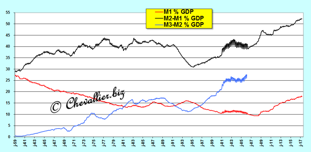
The other monetary aggregates M1 and M3-M2, which together with M2-M1 make up the global money supply M3, should not have an effect on growth as long as the money remains healthy, that is, that they are not the source of monetary creation because sound money is the first pillar of Reaganomics said Arthur Laffer.
This rule of the free money supply is close to the old quantitative theory of money, or to the velocity of the monetary circulation (V for Velocity), which reads as follows:
M * V = P * Q where V = GDP / M
For example, in January 1960, the nominal (annualized) GDP was $ 543.3 billion and M2-M1 was $ 158.2 billion, which corresponds to a monetary circulation velocity V = 543.3 / 158.2 to give V = 3.43
As of March 2017, nominal GDP was $ 19,027.6 billion and M2-M1 was $ 9,942.8 billion, resulting in a monetary circulation velocity V = 1.91
Thus, during this period, the velocity of money circulation fell from 3.43 to 1.91 (it’s a multiple, therefore there is no unity), which is logically accompanied by a decline in the growth of Real GDP from 4.3% to 2.4%.
Document 5:
To restore real GDP growth around 4% year-on-year, M2-M1 would therefore need to sharply decrease to restore a circulation rate of around 3.5.
In this case, M2-M1 is expected to amount around $ 5.5 trillion.
Approximately $ 4,400 billion is expected to be released from M2-M1, either to be spent by Americans on consumer goods, investment in durable goods (or) real estate, or invested in business start-ups or securities, which would in all cases stimulate GDP growth.
Everything is coherent.
However, rather than using the concept of monetary velocity, i.e. V = GDP / M, it is preferable to use now its inverse, namely the ratio M / PIB (in percentage), because it is thus easier to highlight the mechanisms of growth and monetary creation and to find their causes and remedies.
This rule of the free money supply has not only a theoretical interest: it is particularly useful for guiding economic policy so that growth and employment reach their optimal potential over the long period.
Thus, for example, the American authorities should encourage Americans to dissaving.
Other examples: Alan Greenspan, who mastered these monetarist concepts, took great care after the Muslim attacks of September 11, 2001, to persuade Americans to continue spending their dollars by traveling, going to restaurants, performing, shopping and leisure centers so that GDP growth does not falter.
He acted to keep Americans confident in the future and not to increase their savings.
On other hand, in a comparable situation, after the Paris and Nice bombings perpetrated by Muslims, French authorities increased the reactions of defiance and fear by showing a war situation with soldiers patrolling in arms, which has helped to make tourists run away, especially foreign tourists, resulting in a decline in economic activity while growth was already weak elsewhere.
French also spent less, saved more, which did slow down GDP and maintained a large unemployment.
The monetary policy pursued by the Fed after the 2008 financial turmoil, known as Quantitative Easing (QE), was particularly clever because it circulated considerable liquidity available to banks from overfunding cash of large US companies.
Thus, for example, Apple’s cash availability now exceeds $ 250 billion! … which are largely found in bank accounts in the United States, and thus partly placed at the Fed which circulated this sleeping money (i.e. previously unused) by investing it in Treasuries and mortgage-backed securities.
The ECB’s EQ policy is totally different from that of the Fed and has no positive effect because the ECB does not have reserves: it lends hundreds of billions of euros to banks that place them back to the ECB that uses them to acquire euro area treasury bonds.
These are large-scale deceptions that only increase the money supply (in M3-M2) and thus contribute paradoxically to reducing GDP growth!

No comment ? 🙂
Lost in translation 😀
@Julien
« Lost in translation 😀 »
No ! It’s the same story…
off topic :
Bit Coin 2,425$, Next Round is On ?